Current SADA Webpage Vistors

Previous SADA Webpage Visitors

Spatial Analysis and Decision Assistance

Miscellaneous Spatial Tools

The following is a laundry list (not exhaustive) of spatial tools not covered in the other major links of the website.

Automated File Creation

It is often the case that SADA user's retrieve information from a centralized database system within their company, university, or government agency. In version 5.0, we have provided documentation in the user's guide and help file about how IT managers can make simple modifications to their systems to automatically dump data into a SADA file. A small bit of programming by your IT folks is required to create a toolbar button or menu item that will create a simple parameter file that tells SADA how the data should be received and asks SADA to automatically create a file with the data already imported and ready to go. Some commercial databases such as EQuIS have already taken advantage of this new feature.

Model Storage/Import/Export

In versions 1-4 of SADA, users had to regenerate the model each time they wanted to reproduce the result. Now in SADA you can create a 2d or 3d model and store it as a static model that you can recall at anytime. This model can be used in any other part of the software such as decision analysis or sample design as it normally would. In the same manner, users can now import 2d and 3d models into SADA using some industry standard formats (ASCII Grid/FLOAT GRID/DEM) for 2d raster results and a very simple 3d format for 3d results that can acommodate for regular or irregular depth intervals. SADA can export to these same formats as well.

Data Thinning

In an effort to make the import of extremely large data sets tractable (e.g. dense geophysical data sets), SADA will permit users to thin the data somewhat to make visualization and exploration of the data tractable. If a single data set (one contaminant) has many, many points or if an import model has a dense grid definition sada will prompt for an thinning to be implemented. Users can elect not to thin. In the following image a Digital Elevation Model taken from USGS underwent a thinning of a factor of 4 reducing it form 1.6million pixels. In some cases, thinning may not affect the viability of the data. Only the analyst can make this decision.

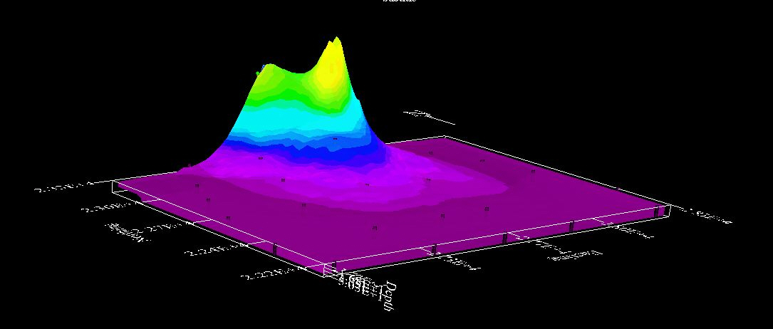
Elevation

SADA 5 is the first version to incorporate elevation. At this point, elevation is implemented in the 3d viewer only, and only after the modeling has been completed. When elevation is incorporated, SADA first models the spatial attributes as depth below surface rather than elevation. Then in the visualization, the points/grid cells are positioned correctly with respect to elevation. This amounts to a shifting of cell blocks and points and not the generation of an elevation surface on top of the 3d model. This is a feature we hope to include in the next version. In the following image, we see an isosurface image of attribute values adjusted for elevation. In this case the attribute is in fact elevation so the colors and height are correlated. The visual result here is quite sufficient but his may vary depending on your application. In particular a 2d model (while accurate) will not present well when adjusted for elevation. We recommend that you export to a package that can produce high quality 3d/elevation images.

Vertical Profiles

You can now view vertical profiles in SADA. The following is a single vertical profiles selected with the click of a mouse from a 3d dataset. Multiple profiles can be viewed as well.

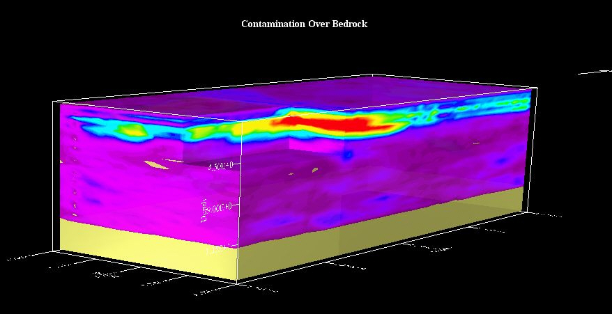
Custom Modeling Features

With stored or imported models (see above) you can now apply a wide array of common algebraic and arithmetic functions to the model results at the cell level. In fact, it is possible to build complex functions that can further extend SADA to very specific situations. In addition, a host of standard "GIS" map manipulation tools are now available such as cutaway rules, merge rules, replacement rules, conversion rules, and so forth. Finally, you can use these rules between maps as well to combine different model features together. Consider for example in the following image the union of a 3d contaminant model with a 3d geologic model showing bedrock position.

In this image a function is applied to the map to create a new map. This new map can then be entered into any post modeling exercises such as decision analysis and sample design.

In this image a categorical conversion rule has been applied.

In this image a cutaway rule based on values was applied.

In this image a smoothing/filter was applied.

User Defined Maps

Users can also create their own custom maps by hand by essentially drawing the maps by hand or in combination with the custom tools (see above) to process a complex result. These can be very useful in communicating spatial organization (for example representative model of subsurface geology or a priori knowledg about contaminant location). These custom maps can be used as secondary forms of information in the multi-variate geostatisical modeling and in some initial, targeted sampling designs.

Polygon Volume/Area

Users can now calculate the area/volume of polygons or other shapes they have drawn. Useful in desiging remedial designs manually.