Welcome to SADA Version 4. A great deal of change has occurred between Version 3 and 4, primarily in the interface. This quick start tutorial is designed to show you how to get around in SADA 4, covering some of the most commonly used functions. This tutorial is not intended to replace the help file, but it can get you up and going much faster.
Overview
First, let’s cover the new interface. After a few moments, we’ll be off and running. The main idea behind the new version 4 interface is to navigate users through the many and often complex functions with simple, everyday language and by presenting only those items relevant to the current task. To accomplish this, Version 4 uses a "steps" approach. SADA will show you the major steps required to accomplish most every major function or model available. The "interview list" contains these major functions, with everything from simple data plots to contour maps to secondary sampling strategies. They appear with plain English names such as "Plot my data", "Draw an area of concern map", and "Develop a new sample design". Below the interview list is a blue box called the steps window that contains all the steps you’ll need to accomplish the major function. When you switch between major functions or interviews, the steps change accordingly. Many of the steps are redundant, appearing in multiple functions.
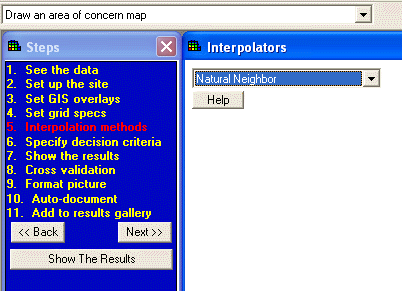
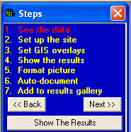
Consider drawing an area of concern map. The following steps appear.
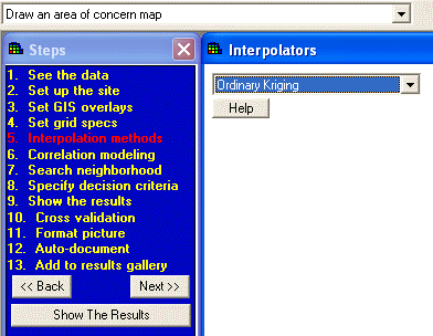
To go to any step, simply click on the item in the list. The steps you see are not only dependent on the major function but on choices you may make within the steps themselves. For example, if we switch the interpolation method from natural neighbor to ordinary kriging (step 6), two new steps appear: Correlation modeling and Search Neighborhood. This is because the ordinary kriging model requires these parameter before it can execute its part of the process. Don’t worry about what these parameters mean right now.
Remember that steps represent an action, decision, or model that needs to be addressed as part of accomplishing the major task. Therefore, associated with each step are a set of options or parameters. These appear to the right of the steps (where natural neighbor and ordinary kriging appear) in the parameters window.
For the area of concern map, clicking on Correlation modeling (step 7) will present you the following information in the parameters window.
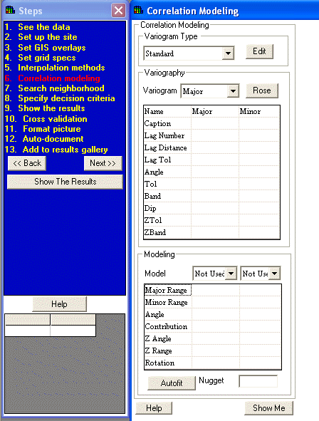
Although the window is mostly blank, we can see what is needed to finish this step. To get help on these parameters, press the help button and SADA will take you to the relevant section of the help file.
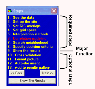
Notice that the steps are really in two major parts. First are the steps leading up to Show the results (Step 9 here). Show the results executes the major task. In this case, it will attempt to create an area of concern map. If you haven’t filled out all the information in the steps leading up to Show the Results, SADA will stop and inform you. Note that you don’t have to complete the steps in order, nor do you have to proceed through each step every time you want to create a new map. The steps following Show the results are simply actions you can take on the result itself. For example, you can format the map, document it, or store it in the results gallery.
There are actually hundreds of parameters or options within the SADA software. Notice that SADA only presents those parameters needed to complete each task.
Get Started
Assuming you’ve installed SADA 4 on your machine, go ahead and start it. You’ll get this screen.
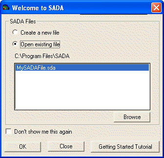
This is a shortcut for opening or creating a new SADA file. (These options are repeated in the File Menu.)
SADA files contain everything you need concerning your data set, such as data sets, model parameters, graphical preferences and so forth. Once you’ve created a SADA file, you can pass it to other SADA 4 users, and they can view the work you’ve done. Later, we’ll learn how to create a new SADA file. (Sorry Version 3 users, SADA 4 is not backwards compatible to earlier SADA file types.)
Double Click on MySADAFile.sda. When the file opens you’ll see the following.
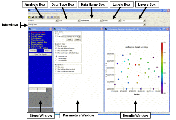
All the major functions are in the interviews list. The blue window on the left is the steps window. Here is where you’ll see all the steps needed to accomplish the major function plus extra steps to post-process the results. Depending on the step selected, the middle window (the parameters window) shows the associated parameters or options. The window on the far right is where you’ll see your results (the graphics window).
Along the top are the same kind of boxes from Version 3. The first box is the analysis box (more later). The second box, which used to be called the media, is now ambiguously called the data type box; it stores all kinds of data types, some of which are not associated with a media. The third box is the data name box. For Version 3 users, it’s the same as the contaminant names box. The label box is next. The final box is the vertical layer box (more on this later).
Click on the interview box and use the scroll bar to display a list of all the functions in version 4.
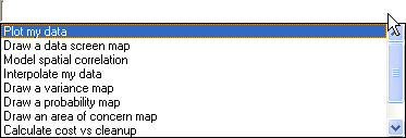
Let’s start with "Plot my data" and take a look at the steps associated with it.
See the Data
For almost all interviews, you’ll see the same first 3 steps: See the data, Set up the site, and set GIS overlays. Click on See the data. The parameters window shows the following.
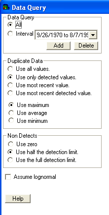
Here is where you can set some standard options regarding sample dates, duplicates, and methods for dealing with non detects.
Set up the site
Click on Set up the site. You should see this in the parameters window.
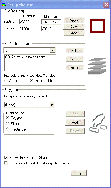
This step is where you set the site boundary, set vertical layers, and create polygons.
Vertical Layers
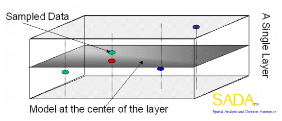
If you have (or will have) three dimensional data, this step allows you to setup 2d slices of the data in the vertical direction. New in Version 4, you can have irregularly spaced layers such as 0-1, 1-4, and 4-8, and SADA will be able to use them in either the data or 3d model world. Also, SADA is more strict on the boundaries of its layers. Previously SADA treated layers as such: 0<=z<=1 and 1 <= z <= 4. Note that a data point could show up on both layers if z = 1. Behind the scenes SADA knew there was only one point at z = 1; however, it did show up on two layers. Version 4 treats layer as such: 0<=z<1, 1<=z<4.
Also on this window are the options to use either the center or top of the layer as the location for estimation or sample design. More on this in the help file. Most people use "In the middle".
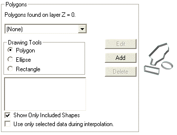
Back in the Steps window, click on Set Polygons to display the following in the parameters window.

Polygons
Polygons have come along way since Version 3. For newcomers, a polygon tool is basically used to focus your analysis by sub-setting areas of your site. Once you’ve drawn a polygon, all analyses will occur only within the boundaries of that polygon. In version 4, you can draw polygons, ellipses, and rectangles.
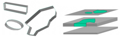
These shape structures are organized in layers (i.e., a collection of polygons can be drawn on each layer). In Version 4, these polygon layers are maintained separately from the vertical layers. That way you can rearrange your vertical layers, delete them, or add them without destroying your polygon designs. In a way, polygon layers in SADA are like GIS layers that can be assigned to specific vertical layers.
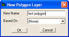
Click the Add button. You will see a New Polygon Layer box. Type MyPolygon into the New Name box and set the Based On box to (None) so it will be a completely new polygon layer. If another polygon layer name was found in the Based On box, then SADA would essentially create a copy of that polygon layer to edit. Press OK.
SADA asks you if want to apply this polygon design to all vertical layers.
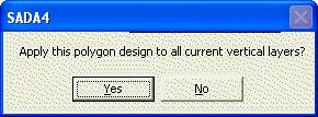
In many applications, users just want their polygon to cut through all their vertical layers. Just answer Yes, and the polygon design will be applied to all current vertical layers. If you answer No, it will only be applied to the layer currently selected. You could then switch to another layer and apply a different polygon design. It doesn’t really matter here, because we only have on layer anyway, but go ahead and press Yes.
You should see MyPolygon in the Polygon Layers box on the parameters window. To add some shapes to your polygon layer, click on Edit. The word Edit turns to Done and virtually everything is disabled. SADA is waiting on you to draw and won’t permit you to click on anything else until you are done drawing. Choose the Polygon option.
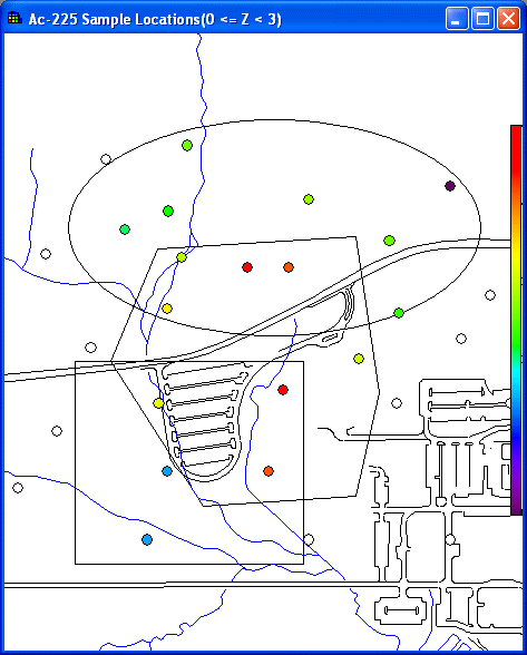
Over in the graphics window, just start clicking around on the screen and you’ll start drawing. To complete the polygon, double click.
To draw an ellipse, choose the ellipse button. Left mouse click on the results window, hold the mouse down, and drag the ellipse open. Release the mouse to finish the ellipse. The same thing works for the rectangle. If you mess up drawing, just double click on the polygon you wish to correct and blue vertices will appear. You can move them around or delete them by left mouse clicking into them. The selected vertex will turn red. Move it or press the delete button. Note that you can’t delete just one vertex of an ellipse. If you want to move or delete the entire shape, right mouse click on one of the shapes. All the vertices turn red, and you can move the entire shape or delete the entire shape by pressing the delete key. When you’re finished press Done.
For now let’s switch back to (none) in the polygon layers list box.
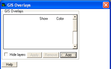
Set GIS Overlays
For now, let’s just leave a single 2d layer at Z = 0 and press Set GIS overlays to display the following.
SADA can now import both dxf and ArcGIS shape file layers. Click on Add, switch the file type to .dxf, and choose Roads.dxf.
Press Open to close this window. Then press Apply on the parameters window for the overlays to appear in the graphics window.
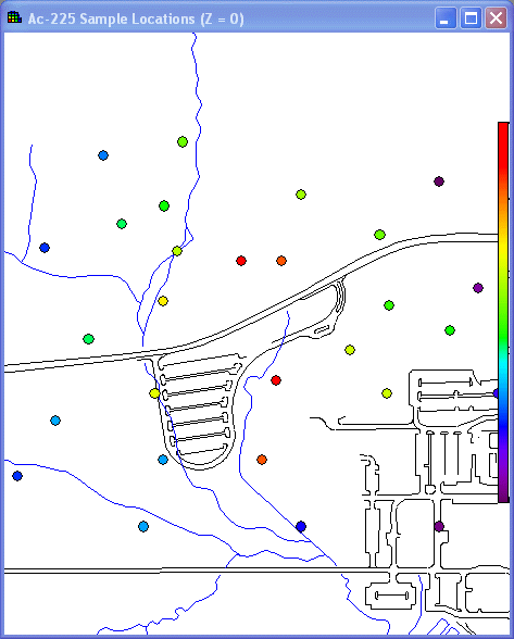
Press the save button to keep this update in your SADA file. ![]()
Show the Results
You can either click on the Show The Results step or press the Show The Results button. SADA will then attempt to execute the model or function found in the interview list. In this case, it’s just a data plot. Later on, it’ll create more excitement.
Format the Picture
Now we’re getting into post-processing steps. Click on Format the Picture to see the options for formatting your result.
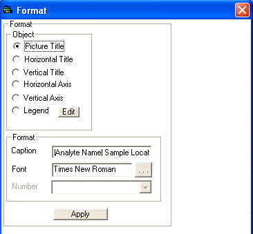
At the top, click on the object you want to format. The caption, font, and number change accordingly. Make your changes and hit apply. Some of these, such as horizontal axis, don’t really apply when you have a GIS view up. They are really intended for the simple XY views.
Auto-Documentation
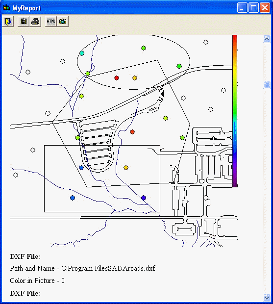
This step will document all the "ingredients" that comprise the current picture in the graphics window, such as model, parameters, assumptions, and various decisions. By pressing Update, SADA will create a report for you and dump all this information into it. The report will actually be an HTML file, which can be opened up in Word, Word Perfect, or any browser. Click on the Auto-Document step and the parameters window changes.
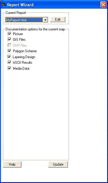
Since we only have a data plot in the graphics window, there aren’t too many elements to document. To create a new report, click on Edit.
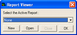
Click on New. Type in MyReport in the space provided and press OK. SADA will create a subdirectory with the name of your report. Just like a website, all pictures in your report will be included with the report file in this subdirectory.
Then, check off all the options in the parameters window. Press Update. Voila!
For more help on Auto-documentation, see the help file. Deselect Show Report Viewer under the Reports menu or click on the Close Viewer Button on the Report Viewer’s toolbar ![]() to close the viewer.
to close the viewer.
Add To Results Gallery
In version 4, you can now save your result into the results gallery. This allows you to see the result without having to re-generate it each time. (Version 3 users might appreciate this). For results that require a great deal of computational time, this can speed things up a great deal. Once you have your result in the results gallery, you can still perform some functions, such as format it, spin it (in 3d viewer), and so forth.
Click on the Add To Results step. The parameter window shows the following.

Type "My Result" in the box next to Save result as…. and press Add. SADA presents the following message.

Press OK. This result is now listed in the data type box (old media box). Change it from Soil to Results Gallery to see "My Result" in the data name box.

The result also appears in the graphics window, and the steps window changes. Note: there are only a few things you can do with result.
We’ve now covered the most common steps found in SADA. You’ll see these steps again and again for almost every interview. The good news is that SADA remembers you’ve completed them and keeps your last choices, even when you switch between major functions. That way you don’t really have to complete the steps over again. This really reduces the list of steps you need to revisit multiple times to just 2 or 3.
Now try some of the other functions. These may require knowledge of the models before you can really use them. Refer to the help file for a detailed explanation of these major functions, their steps, and the parameters associated with them.
Try another simple map. Switch from Results Gallery to Soil. In the interview box, select "Draw a data screen map". This function will highlight any data points that are in excess of a given threshold value. Notice that the steps are the same, but when you press the Show The Results button, SADA asks for a decision goal.

It’s really asking you what sampled value is the highest you would want to see. SADA will then highlight those data points that exceed that value. Type in a 3, press OK, and SADA puts boxes around all those points that exceed a value of 3.

Now let’s create SADA files from scratch.
Create your own files
There are two types of files that SADA can create: standard SADA files, where you have some data to import, and empty files. An empty file has no data but can be used to create initial sample designs.
Creating Empty SADA files
Select File -> New. If you have a file open, SADA will ask if you want to save it first. Afterwards you should see the following message.

Click Next>>.

Choose "I don’t have data to import now" and press OK.

Enter MySADAFile.sda for the name of the new file and press Next >>. SADA presents the empty plot in the graphics window.

Not much to look at because you don’t have any data. The interview box only contains "Draw an Empty Plot" and "Develop Sample Design". In the graphics window, SADA has created default spatial extents from 0 to 1 in both the easting and northing directions. If we click on the Set Vertical Layers step, we see that a default layer of z=0 has been created. Now, click on Set GIS Overlays to add the roads.dxf layer (see above).
Now, SADA presents the user with the following message.

SADA recognizes that the roads.dxf spatial extent is much different than the 0 – 1 extents. It is simply warning us that this might cause trouble. This message appears for both standard and empty SADA files under these circumstances. Press OK.
In the next message box, SADA has recognized that this is an empty SADA file and you may wish to base your spatial extents on the imported dxf layer.

Click Yes. The GIS layer is listed in the parameters window.

Now press Apply, and the graphics window will change dramatically.

Furthermore, when you click on Set Site Boundaries, you’ll see that SADA has updated the spatial extents.
Let’s suppose now that the entire GIS layer is not really your site. If you know the coordinates of the site, you can enter them by hand. You can also use the draw button to tell SADA where your site is. Click on Draw. In the graphics window, left mouse click somewhere and hold it down. Now drag open the rectangle associated with your site. When you release the mouse, SADA now recognizes this area as where you want to perform your actions.

The selected site is zoomed and centered in the graphics window. (Note that it might be a different location than in the following figure).

The Set Polygon step works the same way in an empty file.
The Import Sampled Data step takes you to the import wizard to import data. See the help file for more information.
The Setup Geobayesian model is explained in detail in the help file and is intended for advanced users.
The last two steps, Format Picture and Auto-Document, are the same as before.
In the interview box, now select "Develop a sample design".

The steps look much the same but now we have a new step called set design parameters. Click on this step to select a sample design.

In the parameters window, the sample designs available for empty files will be listed in the Sample Design box.

To demonstrate how sample designs work, select Simple Random. The parameters window will look like the following.
For now, type in 25 under "Number of Samples" next to the "You Pick" option. In the steps window, press the Show The Results button. You just created an initial sample design in SADA.

To export these coordinates out to your sampling team, press the export button  and SADA will ask for a file name.

Type in MySampleDesign and press Save. SADA will then export your new sample coordinates to a csv file. This file may then be used by your sampling team to navigate using GPS or another locater device. Please refer to the help file for full explanations of all the other sample designs.
Create a Standard SADA file
Close your empty file. Select File - >New. The first couple of windows should be familiar.

Press Next >> to continue, and this time select "I have data to import now." Press OK.

SADA opens the File Selection window. At this point, enter the name of your new SADA file into the first textbox. Then, enter twodimensional.csv into the second textbox. Twodimensional.csv is a comma delimited text file that contains the data we want to import. Press Next>> for SADA to convert your data file into this new SADA file. Note: the external file itself is not affected by the conversion process.
The next step in the process is to identify the columns of information in the ascii data file and match these columns of information to information categories that are required or may be useful in SADA. SADA scans the text file for column headers and applies default matches to these information categories. The results are shown in the Matching Headers with Categories window. If a column is mismatched with an information category type, Select a new column header by pressing the down arrow and highlighting the new column header.
Required information categories are followed by an (*) and must be assigned to a column in the ascii data file. A category is not assigned if the (none) option is selected in the drop down box. The Depth category is required only when data exist at varying depths. If the Detect Qualifier is not assigned, the data are assumed to be all detects. If the media column is not assigned, SADA adds an artificial media column titled ‘Basic’.
WARNING:
If Media ID, which denotes the type of media the contaminants are sampled in (e.g. soil or groundwater), is not defined, then the human health risk and/or ecological risk modules cannot be setup later. The media is a information category critical to the risk modules. Also, SADA expects certain units for measured values in the risk modules.

After the columns have been set, press Next>>. SADA begins the conversion process and presents the data is it will be imported into the Data Editor.

The Data Editor is a simple spreadsheet that shows how SADA views the data as it's being imported. It provides the user a chance to identify errors in the data set and correct them during the import process. At this point, the Data Editor is very simple in functionality and is designed to correct minor errors in the data. If for some reason the data import appears to be largely different than the user intended, the exact cause should be identified outside of SADA and the setup repeated.
SADA highlights cells with red if they contain an unacceptable value for SADA. In the example above, the northing column contains a value of NA. Since SADA requires numerical values for every northing entry, the cell is now red. To determine the exact error, place the mouse over the red cell and the yellow text box near the top explains the problem with the entry.
Once the spreadsheet contains no red cells, the process may continue. Near the top is a checkbox called Automatic Error Checking. It is recommended that this box remain checked. When unchecked, SADA is no longer looking for mistakes as you type. Under these conditions, you must press the Check Errors button at the bottom of the page to run the check. It may be preferable to uncheck the Automatic Error Checking box and use Check Errors later when the user is entering or pasting large amounts of data and does not wish the process to be slowed by SADA checking values as they are entered. However, generally during the import process it should remain checked. If there are many errors or the file is large, use the Find Next Error button for SADA to locate the next error.
After scanning in the contaminants, SADA checks for duplicate values. Duplicate values are resolved based on the criteria defined for the data query parameters, visible when See the Data is selected from the Steps Window.
Click Submit after all errors have been corrected. The SADA file is now successfully created and is automatically opened.

Before a data set can be converted into a SADA file, it must adhere to the following requirements:
1. The data set must be in comma delimited text or in Microsoft Access.
2. The file must include at least four columns, in any order, that contain the analyte name, easting coordinate, northing coordinate, and sample value. If the data are taken over depth, an additional column with the depth value is required. No empty values are allowed for any of these columns, and non-numerical values are not permitted for any coordinate or sample value.
3. Columns containing CAS Numbers, Detect Qualifiers, Media Identification, and date are optional. Additional columns are accepted; however, the total number of columns may not exceed 250. CAS Numbers are accepted with or without dashes and without trailing or leading zero values. Valid detection qualifiers consist of only 0 and 1, non-detect and detect respectively. Proper media identification qualifiers are as follows: Soil – SO, Sediment – SD, Groundwater – GW, Surface water – SW, Air – AIR, Biota – BIO, and Background – Background. Proper date format is mm/dd/yy.
4. All columns must have a title row. Punctuation is not allowed in the title names.
5. If risk assessments are part of the analysis (either human health or ecological), then the concentration values are expected to be:
Soil, Sediment, and Biota: mg/kg for nonradionuclides, pCi/g for radionuclides
Surface/Groundwater: mg/L for nonradionuclides, pCi/L for radionuclides
In addition, a Media Identification column is required for setting up the human health risk or ecological risk modules.
6. Quotation marks are located only around items that contain a comma. SADA accepts quotations as field delimiters and may get fields out of order. For example, the value Sample located on "C" Street is accepted as three column values: Sample located, C, and Street. Conversely, Arsenic, Inorganic must be enclosed in quotes or SADA will read it as two field values: Arsenic and Inorganic. The proper way to store the field value is "Arsenic, Inorganic".
After you’ve created the SADA file, try each of the steps under Plot the Data that you saw in the first part of the tutorial. Also try out the other major functions in the interview list. More information can be found in the help file.
Setting up Analyses (Human Health, Ecological, MARSSIM, Custom)
SADA arranges itself according to the major function selected in the interview box. The interview box, however, is affected by the type of analysis. Up until this point, only the General analysis has been used. When you first create a standard SADA file, General is the only item found in the analysis box. You can also conduct Human Health, Ecological, MARSSIM, and Custom analyses, but they must first be set up.
Each of these analyses has a very similar setup routine and looks outside of SADA to a corresponding database packed with SADA. These databases, such as ecotox_data.mdb, ToxicologicalProfiles.mdb, and MARSSIM.mdb, all contain contaminant-specific information necessary to run the analysis. For this reason, each setup require you to match contaminants found in your SADA file to those found in the database. SADA tries to help with the matching. In most cases, this is all you really have to do to setup any given analysis. As an example, we’ll set up the human health risk now.
Setting Up Human Health Risk
All analysis setups can be accessed through the Setup menu. This menu is only active for standard SADA files (those that have data).

To initiate the Risk Setup Wizard, select Human Health Risk from the Setup menu of the main window.

Select Yes. (Select No to cancel the setup process.) In the next window, SADA needs the names of the supporting toxicological profiles and scenario parameters databases. The toxicological database contains health related information about individual contaminants. The scenario database contains parameters regarding the human receptor exposure patterns. SADA comes with two default databases. The ToxicologicalProfiles.mdb comes from Oak Ridge National Laboratory’s Risk Assessment Information System (RAIS). This toxicological database is maintained regularly, and recent versions of the database can be downloaded from the SADA home page in a SADA compatible format. The toxicity values were compiled from EPA's Integrated Risk Information System (IRIS) and Health Effects Assessment Summary Tables (HEAST), derived from values found in these EPA sources, or provided after contacting EPA. The scenario parameters database, ScenarioParameters.mdb, contains default parameters established for the Oak Ridge Reservation and may need customizing for your particular site.

Once the databases have been selected, press Next >> to continue.
SADA now attempts to match each contaminant in your file with a contaminant found in the toxicological database. SADA searches by CAS number first (if available) and then by name. If the CAS number and name match exactly, SADA classifies it as Matched. If only the Name or the CAS number match, then the classification is Partial Match. Finally, if no match is found for either, the classification is No Match. These three classifications are presented in the Contaminant Identification Results Window.

On the left side of the window, your contaminants have been divided into the three categories. To view a resulting match for any contaminant, click on the down arrow and select your contaminant from the resulting drop down list. The corresponding selection on the right hand side will change to show SADA’s match for your contaminant. If the match is acceptable, press the Register button. If all matches within a category are acceptable, press Register All. To unregister a matched pair(s), select the pair(s) in the registered contaminants box and press Unregister. Your contaminants will return to their original classification with their original match.
If no match is available for some of your contaminants, you may leave them as unregistered. Later, if the toxicological information becomes available, you may link these contaminants (or re-link registered contaminants) separately without setting up the entire risk module again. See Toxicological Links. For this example, just select "Register All" for both Matched and Partial Match. Press Next>> to conclude setting up the risk module.
Once the module is complete, Human Health analysis will appear in the analysis box. Additionally, a Human Health menu will be visible in SADA when this analysis is selected from the combo box.
Press the save button  to save these setup changes.

What kind of impact does setting up an analysis make? Most noticeably, another menu item named after the analysis appears at the top (the exception is MARSSIM). This menu contains actions and settings specific to human health risk. Find out more about these in the help file.

Secondly, the interview list is changed to only include the models available for a human health analysis.
Note that we now have "Draw a point risk map" and "Draw a contoured risk map".
Other important changes have occurred as well. For example, when you perform a simple "data screen map", SADA will ask you for human health landuse/pathway scenario instead of a user-defined value. To test this, switch the interview choice to "Draw a data screen map".

The steps look the same as they did under General; however, when you press the Show The Results button SADA now asks for a landuse/pathway scenario.

Accept the default and press OK. SADA runs the human health preliminary remediation goal model (see the help file) to come up with a threshold concentration value called the PRG.

SADA will now highlight all those data points exceeding this value.

Summary
This covers the primary basics for navigating through SADA version 4. You are encouraged to read the help file, return to the website for supplementary materials, and to attend trainings as they become available.
Remember, you can report any suspected errors or make suggestions by e-mailing sada@tiem.utk.edu or selecting Report a Problem from the About menu.